Geographically Weighted Regression in SAGA

Since I mentioned kernels last week, I figured this would be a good time to go over the geographically weighted regression (GWR) procedure in SAGA. Once again, I don’t have good example data I can post online for this topic, so you’ll have to forgive the lack of pictures.

GWR is an interesting method with lots of applications. GWR is different from other techniques because it allows the relationships between covariates to vary spatially. For some research questions, it is helpful to use GWR to see where certain predictor variables are more or less important for predicting an outcome. GWR is flexible enough that you can analyze your data at many scales, and see error estimates and at many scales too.

Today we’re using GWR for interpolation. If you haven’t used SAGA before, I recommend starting with this SAGA Basics post. You’ll need to know how to open raster data and point data.

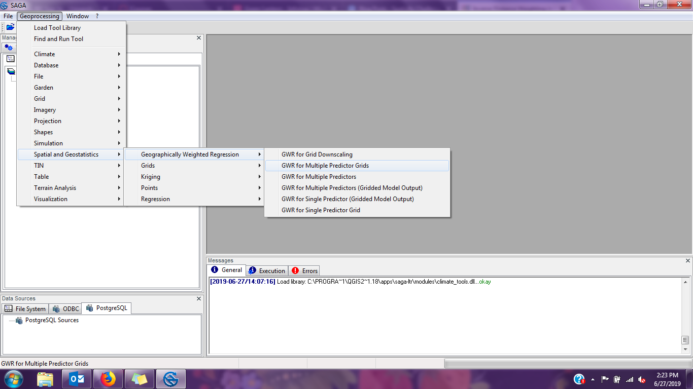
In today’s hypothetical interpolation example, let’s say you’re trying to get a map of soil lead concentration surrounding the site of an old factory. You have soil test results with lead levels stored as point data, and raster layers of historic rainfall and elevation. After opening your data sources, you need to open the GWR pop up menu by going to Geoprocessing > Spatial and Geostatistics > GWR. Since we have two different raster layers (rainfall and elevation), you’ll want to use GWR for multiple grid predictors.

Once you’re in the GWR window, it looks pretty similar to other procedures in SAGA. Select your grid system and your data layers. Be careful to select not just the right point file, but also the correct attribute within this point data. I also like to create a layer of residual values at the study spot– this is useful if you want to calculate RMSE or other global error metrics. If you want to see how the parameters for each variable changes across your study space, click the checkbox next to “Output of Regression Parameters.”

From here you’re into the kernel bit! The weighting function has a variety of options like we talked about in this post about kernels. SAGA will suggest a bandwidth based on the grid system size and resolution, but you can also input your own. The search range is a cut off that helps determine how far the algorithm will look for points to include if you use a variable bandwidth. I’ve always used global searches, but I bet this would be good for really excessively large maps.

From here you can run the GWR procedure, output your data as a TIFF if you so choose (directions buried in here), and look at your pretty map in SAGA. Thanks for reading, and good luck map making!